Файл:Karmarkar.svg

Размер этого PNG-превью для исходного SVG-файла: 720 × 540 пкс. Другие разрешения: 320 × 240 пкс | 640 × 480 пкс | 1024 × 768 пкс | 1280 × 960 пкс | 2560 × 1920 пкс.
Исходный файл (SVG-файл, номинально 720 × 540 пкс, размер файла: 43 Кб)
Этот файл находится на Викискладе. Сведения о нём показаны ниже.
Викисклад — централизованное хранилище для свободных файлов, используемых в проектах Викимедиа.
|
Краткое описание
| Описание |
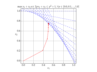
English: Solution of example LP in Karmarkar's algorithm.
Blue lines show the constraints, Red shows each iteration of the algorithm. |
| Дата | |
| Источник | Собственная работа |
| Автор | Gjacquenot |
Лицензирование
Я, владелец авторских прав на это произведение, добровольно публикую его на условиях следующей лицензии:
Этот файл доступен по лицензии Creative Commons Attribution-Share Alike 4.0 International
- Вы можете свободно:
- делиться произведением – копировать, распространять и передавать данное произведение
- создавать производные – переделывать данное произведение
- При соблюдении следующих условий:
- атрибуция – Вы должны указать авторство, предоставить ссылку на лицензию и указать, внёс ли автор какие-либо изменения. Это можно сделать любым разумным способом, но не создавая впечатление, что лицензиат поддерживает вас или использование вами данного произведения.
- распространение на тех же условиях – Если вы изменяете, преобразуете или создаёте иное произведение на основе данного, то обязаны использовать лицензию исходного произведения или лицензию, совместимую с исходной.
Source code (Python)
#!/usr/bin/env python
# -*- coding: utf-8 -*-
#
# Python script to illustrate the convergence of Karmarkar's algorithm on
# a linear programming problem.
#
# http://en.wikipedia.org/wiki/Karmarkar%27s_algorithm
#
# Karmarkar's algorithm is an algorithm introduced by Narendra Karmarkar in 1984
# for solving linear programming problems. It was the first reasonably efficient
# algorithm that solves these problems in polynomial time.
#
# Karmarkar's algorithm falls within the class of interior point methods: the
# current guess for the solution does not follow the boundary of the feasible
# set as in the simplex method, but it moves through the interior of the feasible
# region, improving the approximation of the optimal solution by a definite
# fraction with every iteration, and converging to an optimal solution with
# rational data.
#
# Guillaume Jacquenot
# 2015-05-03
# CC-BY-SA

import numpy as np
import matplotlib
from matplotlib.pyplot import figure, show, rc, grid

class ProblemInstance():
    def __init__(self):
        n = 2
        m = 11
        self.A = np.zeros((m,n))
        self.B = np.zeros((m,1))
        self.C = np.array([[1],[1]])
        self.A[:,1] = 1
        for i in range(11):
            p = 0.1*i
            self.A[i,0] = 2.0*p
            self.B[i,0] = p*p + 1.0

class KarmarkarAlgorithm():
    def __init__(self,A,B,C):
        self.maxIterations = 100
        self.A = np.copy(A)
        self.B = np.copy(B)
        self.C = np.copy(C)
        self.n = len(C)
        self.m = len(B)
        self.AT = A.transpose()
        self.XT = None

    def isConvergeCriteronSatisfied(self, epsilon = 1e-8):
        if np.size(self.XT,1)<2:
            return False
        if np.linalg.norm(self.XT[:,-1]-self.XT[:,-2],2) < epsilon:
            return True

    def solve(self, X0=None):
        # No check is made for unbounded problem
        if X0 is None:
            X0 = np.zeros((self.n,1))
        k = 0
        X = np.copy(X0)
        self.XT = np.copy(X0)
        gamma = 0.5
        for _ in range(self.maxIterations):
            if self.isConvergeCriteronSatisfied():
                break
            V = self.B-np.dot(self.A,X)
            VM2 = np.linalg.matrix_power(np.diagflat(V),-2)
            hx = np.dot(np.linalg.matrix_power(np.dot(np.dot(self.AT,VM2),self.A),-1),self.C)
            hv = -np.dot(self.A,hx)
            coeff = np.infty
            for p in range(self.m):
                if hv[p,0]<0:
                    coeff = np.min((coeff,-V[p,0]/hv[p,0]))
            alpha = gamma * coeff
            X += alpha*hx
            self.XT = np.concatenate((self.XT,X),axis=1)

    def makePlot(self,outputFilename = r'Karmarkar.svg', xs=-0.05, xe=+1.05):
        rc('grid', linewidth = 1, linestyle = '-', color = '#a0a0a0')
        rc('xtick', labelsize = 15)
        rc('ytick', labelsize = 15)
        rc('font',**{'family':'serif','serif':['Palatino'],'size':15})
        rc('text', usetex=True)

        fig = figure()
        ax = fig.add_axes([0.12, 0.12, 0.76, 0.76])
        grid(True)
        ylimMin = -0.05
        ylimMax = +1.05
        xsOri = xs
        xeOri = xe
        for i in range(np.size(self.A,0)):
            xs = xsOri
            xe = xeOri
            a = -self.A[i,0]/self.A[i,1]
            b = +self.B[i,0]/self.A[i,1]
            ys = a*xs+b
            ye = a*xe+b
            if ys>ylimMax:
                ys = ylimMax
                xs = (ylimMax-b)/a
            if ye<ylimMin:
                ye = ylimMin
                xe = (ylimMin-b)/a
            ax.plot([xs,xe], [ys,ye], \
                    lw = 1, ls = '--', color = 'b')
        ax.set_xlim((xs,xe))
        ax.plot(self.XT[0,:], self.XT[1,:], \
                lw = 1, ls = '-', color = 'r', marker = '.')
        ax.plot(self.XT[0,-1], self.XT[1,-1], \
                lw = 1, ls = '-', color = 'r', marker = 'o')
        ax.set_xlim((ylimMin,ylimMax))
        ax.set_ylim((ylimMin,ylimMax))
        ax.set_aspect('equal')
        ax.set_xlabel('$x_1$',rotation = 0)
        ax.set_ylabel('$x_2$',rotation = 0)
        ax.set_title(r'$\max x_1+x_2\textrm{ s.t. }2px_1+x_2\le p^2+1\textrm{, }\forall p \in [0.0,0.1,...,1.0]$',
                     fontsize=15)
        fig.savefig(outputFilename)
        fig.show()

if __name__ == "__main__":
    p = ProblemInstance()
    k = KarmarkarAlgorithm(p.A,p.B,p.C)
    k.solve(X0 = np.zeros((2,1)))
    k.makePlot(outputFilename = r'Karmarkar.svg', xs=-0.05, xe=+1.05)
История файла
Нажмите на дату/время, чтобы посмотреть файл, который был загружен в тот момент.
| Дата/время | Миниатюра | Размеры | Участник | Примечание | |
|---|---|---|---|---|---|
| текущий | 15:34, 22 ноября 2017 | | 720 × 540 (43 Кб) | DutchCanadian | The right hand side for the constraints appears to be p<sup>2</sup>+1, rather than p<sup>2</sup>, going by both the plot and the code (note the line <tt>self.B[i,0] = p*p + 1.0</tt>). Updated the header line. |
| 19:29, 3 мая 2015 |  | 720 × 540 (41 Кб) | Gjacquenot | Updated constraint display | |
| 19:26, 3 мая 2015 |  | 720 × 540 (41 Кб) | Gjacquenot | Updated constraint display | |
| 19:17, 3 мая 2015 |  | 720 × 540 (41 Кб) | Gjacquenot | Updated constraint display | |
| 18:54, 3 мая 2015 |  | 720 × 540 (41 Кб) | Gjacquenot | User created page with UploadWizard |
Использование файла
Следующая страница использует этот файл:
Глобальное использование файла
Данный файл используется в следующих вики:
- Использование в ar.wikipedia.org
- Использование в en.wikipedia.org
- Использование в fr.wikipedia.org
- Использование в ja.wikipedia.org
- Использование в ko.wikipedia.org
- Использование в pt.wikipedia.org
- Использование в simple.wikipedia.org
- Использование в uk.wikipedia.org
- Использование в zh.wikipedia.org